Introduction to Inverse RL: BC and DAgger.
Behavioral Cloning
We’re given a set of expert demonstrations $\xi \in \Xi$ to determine a policy $\pi$ that imitates the expert, $\pi^*$. In behavioral cloning, we accomplish this through simple supervised learning techniques, where the difference between the learned policy and expert demonstrations are minimized with respect to some metric.
Concretely, the goal is to solve the optimization problem:
\[\hat{\pi}^* = \underset{\text{argmin}}{\pi} \sum_{\xi \in \Xi} \sum_{x \in \xi} L(\pi(x), \pi^*(x))\]where $L$ is the cost function, $\pi^ * (x)$ is the expert’s action at state $x$, and $\hat{\pi}^*$ is the approximated policy.
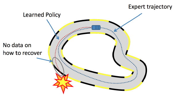
In many cases, expert demonstrations will not be uniformly sampled across the entire state space, and therefore it’s likely that the learned policy will perform poorly when not close to states found in $\xi$. This is particularly true when the expert demonstrations come from a trajectory of sequencial states and actions, such that the distribution of the sampled states $x$ in the dataset is defined by the expert policy.
Then, when an estimated policy $\hat{\pi}^*$ is used in practice it produces its own distribution of states that will be visited, which will likely not be the same as in the expert demonstrations! This distributional mismatch leads to compounding errors, which is a major challenge in imitation learning.
DAgger: Dataset Aggregation
A straightforward solution is to simply collect new expert data as needed. In other words, when the learned policy $\hat{\pi}^*$ leads to states that aren’t in the expert dataset just query the expert for more information!
Data: $\pi^*$
Result: $\hat{\pi}^*$
$\mathcal{D} \leftarrow 0$
Initialize $\hat{\pi}$
For $i = 1$ to $N$ do:
- $\pi_i = \beta_i \pi^* + (1 - \beta_i)\hat{\pi}$
- Rollout policy $\pi_i$ to sample trajectory $\tau = {x_0, x_1,…}$
- Query expert to generate dataset $\mathcal{D}_i = {(x_0, \pi^* (x_0)), (x_1, \pi^* (x_1)), …}$
- Aggregate datasets: $\mathcal{D} \leftarrow \mathcal{D} \cup \mathcal{D}_i$
- Retrain policy $\hat{\pi}$ using aggregated dataset $\mathcal{D}$.
Return $\hat{\pi}$.
This has the advantage of us learning what the expert would do under the data distribution generated by the learner policy. Over time, this process drives the policy to better approximate the true policy as well as reduce the incidence of distributional mismatch. We might imagine that our expert would drive our learner towards certain attractor states, and that this might be learned by our learner.
Me IRL: Themes of Inverse Reinforcement Learning
Three core ideas:
-
Behavioral cloning provides no way to understand the underlying reasons for the expert behavior (no reasoning about outcomes or intentions).
-
The expert might actually be suboptimal.
-
A policy that’s optimal for the expert might not be optimal for the agent if they have different dynamics, morphologies, or capabilities.
In this section, the fundamental concepts will be presented by parameterizing the reward as a linear combination of nonlinear features: \(R(s, a) = w^\intercal \phi(s, a)\)
where $w \in \mathbb{R}^n$ is a weight vector and $\phi(s, a)$ is a feature map. For a given feature map $\phi$, the goal of inverse RL can be simplified to determining the weights $w$. Recall that the total discounted reward under a policy $\pi$ is defined for a time horizon $T$ as:
\[V_T^\pi(s) = \mathbb{E}\left[\sum_{t=0}^{T-1} \gamma^t R(s_t, \pi(x_t)) | s_0 = s\right]\]