Gradient Estimation: Training What You Can’t Backprop Through

Introduction

Neural networks work well through the magic of backpropagation, but there are times when we can’t backpropagate through our layers. Let’s imagine we have a simple problem: We have a Mixture of Experts (MoE) model with a probabilistic routing layer.

To be specific, our routing layer selects one expert to route its computation through.

graph TD A[Input] --> B{Router} B -->|Route 1| C[Expert 1] B -->|Route 2| D[Expert 2] B -->|Route 3| E[Expert 3] C --> F[Output] D --> F E --> F

Our router is a simple linear projection and softmax that takes in our input vector $x \in \mathbb{R}^d$ to produce probability distribution over three experts.

Mathematically, we express this as $p = \text{softmax}(x W_r)$, where $W_r \in \mathbb{R}^{d \times k}$ is our routing matrix. We can sample from this distribution to get a single expert to route to ($i \sim p$), before running the rest of our network as usual ($l_{out} = \text{Expert}_i(x)$).

We have:

Logits: The input x passes through a linear layer to produce logits $l$ for each expert.

\[l = x W_r + b_r\]

Probabilities: The logits are converted to probabilities using softmax.

\[p = \text{softmax}(l)\]

Sampling: An expert index i is sampled from the calculated multinomial distribution with probabilities p.

\[i \sim \text{Multinomial}(p)\]

One-Hot Encoding: We represent the chosen expert i as a one-hot vector y, where the $i$-th element is 1 and the rest are 0.

\[y = \text{One-Hot}(i)\]

Routing: We compute the output of our layer as $l_{out} = \text{Expert}_i (x)$. Mathematically, this is equal to:

\[l_{out} = \sum_{j=1}^k y_j\ \text{Expert}_j(x)\]

Note that there’s a slight mathematical sleight-of-hand here to simplify the STE conceptualization for later on.

Our router normally indexes the expert list to pick one selected expert. Here, I write this as taking the dot product of the one-hot indexing vector with the vector of outputs from all the experts. Effectively, activating all the experts and throwing away all of the outputs except for the one chosen (dot-producting with a one-hot vector) is the same as activating a single expert.

Let’s visualize this computational flow:

graph TD A[Input x] --> B[Linear Layer: xW_r + b_r] B --> C[Logits l] C --> D[Softmax] D --> E[Probabilities p] E --> F[Multinomial Sampling] F --> G[Expert Index i] G --> H[One-Hot Encoding] H --> I[One-Hot Vector y] A --> J[Expert 1] A --> K[Expert 2] A --> L[Expert 3] I --> M[Weighted Sum] J --> M K --> M L --> M M --> N[l_out] style F fill:#ffcccc style G fill:#ffcccc style H fill:#ffcccc

This graph mirrors the sequential math operations outlined above, and I’ve highlighted the nondifferentiable operations in red. Now the problem becomes clear: during the backwards pass, how do we update our routing layer?

The chain rule gives us:

\[\underset{Routing\ Gradient}{\frac{\partial L}{\partial p}} = \left[\underset{\text{Incoming Gradient}}{\frac{\partial L}{\partial y}} \right] \left[\underset{\text{Local Gradient}}{\frac{\partial y}{\partial p}}\right]\]

The issue arises when we try to compute $\frac{\partial y}{\partial p}$. We don’t know whether to upweight or downweight the probability of selecting the expert we selected, as we have no way of computing the counterfactual performance of selecting the other experts. Indeed, torch’s multinomial has no gradient; if we selected our expert using argmax or any other sampling method, we would face the same problem.

If we write out our code in Pytorch and visualize the autograd graph, we can validate that there’s no gradient flow to our routing weights.

Code

import torch
from torch.nn import functional as F

class RoutingLayer(torch.nn.Module):
    def __init__(self, model_dim, num_experts):
        super(RoutingLayer, self).__init__()
        self.model_dim = model_dim
        self.num_experts = num_experts
        self.forward_proj = torch.nn.Linear(model_dim, num_experts)

    def forward(self, x):
        forward_proj = self.forward_proj(x)
        forward_proj = F.softmax(forward_proj, dim=-1)
        chosen_expert = torch.multinomial(forward_proj, 1)
        return chosen_expert

class ExpertLayer(torch.nn.Module):
    def __init__(self, model_dim, num_experts):
        super(ExpertLayer, self).__init__()
        self.model_dim = model_dim
        self.num_experts = num_experts
        self.experts = torch.nn.ModuleList([torch.nn.Linear(model_dim, model_dim) for _ in range(num_experts)])

    def forward(self, x, chosen_expert):
        batch_size = x.shape[0]
        outputs = []
        for i in range(batch_size):
            expert_idx = chosen_expert[i].item()
            outputs.append(self.experts[expert_idx](x[i:i+1]))
        return torch.cat(outputs, dim=0)
    
class RoutingNN(torch.nn.Module):
    def __init__(self, model_dim, num_experts):
        super(RoutingNN, self).__init__()
        self.routing_layer = RoutingLayer(model_dim, num_experts)
        self.expert_layer = ExpertLayer(model_dim, num_experts)

    def forward(self, x):
        chosen_expert = self.routing_layer(x)
        return self.expert_layer(x, chosen_expert)

MODEL_DIM = 8
BATCH_SIZE = 1
NUM_EXPERTS = 3
x = torch.randn(BATCH_SIZE, MODEL_DIM)
model = RoutingNN(model_dim = MODEL_DIM, num_experts = NUM_EXPERTS)

chosen_expert = model.routing_layer(x)
output = model.expert_layer(x, chosen_expert)
loss = output.sum()

from torchviz import make_dot
make_dot(loss, params=dict(model.named_parameters()))

Autograd Routing Graph

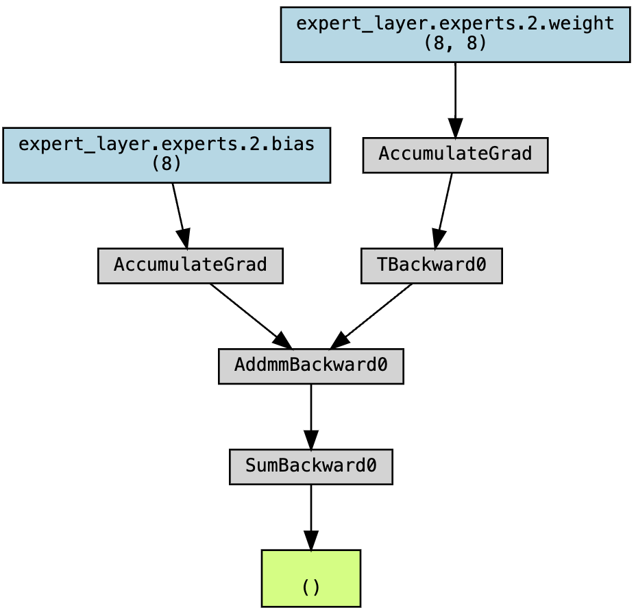
Note that there’s no gradient flow to any blocks with the name prefix routing_layer. For what the autograd compute graph should look like if the routing layer were trainable, see below.

The backprop hack

In the literature, there are a few ways we can backprop through non-differentiable operations. Most of them introduce a surrogate gradient that provides some learning signal and pushes the parameters of the non-differentiable operation in the right direction, and is what we’ll explore for the rest of this post. In the chain rule, the surrogate gradient replaces the local gradient (which is uncomputable). As a whole, this field is called gradient estimation.

Without going too far into the field, here are a few gradient estimation methods:

Straight-Through Estimators (STEs): We pretend that the non-differentiable operation is the identity function during the backwards pass. It’s called “straight-through” because we pass straight through the non-differentiable operations (the three blocks in red above) as if they were not there. In this case, we’d approximate:

\[\frac{\partial L}{\partial p} \approx \frac{\partial L}{\partial y}\]

REINFORCE: We conduct reinforcement learning on the troublesome operation. As you may expect from RL, this gradient estimator is high-variance and can explode your model during training if not properly handled.

\[\nabla_\theta \mathbb{E}[L] = \mathbb{E}\left[\frac{\partial L}{\partial y} \cdot \nabla_\theta \log p_\theta(k|x)\right]\]

Gumbel-Softmax: I’ll cover more on this in another post. This is a biased gradient estimator for argmax that empirically works very well, with the bias-variance tradeoff being tunable via temperature.
Custom estimators: For every common non-differentiable operation, there are tons of papers proposing different functions as gradient estimators. Recent research suggests that the straight-through estimator is approximately as good as any alternative, so try an STE baseline before you go custom.

STEs

Let’s just pretend that the local non-differentiable gradient is 1:

\[\left[\underset{\text{Local Gradient}}{\frac{\partial y}{\partial p}}\right] \approx 1\]

Such that:

\[\underset{\text{Routing Gradient}}{\frac{\partial L}{\partial p}} = \underset{\text{Incoming Gradient}}{\frac{\partial L}{\partial y}}\]

Given how simple this estimation is, does it work?

alt text

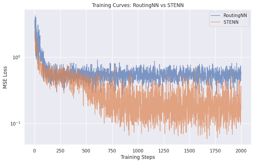
RoutingNN is our routing model defined in the above computational graph, and STENN is the same routing model + STE trick.

Yes.

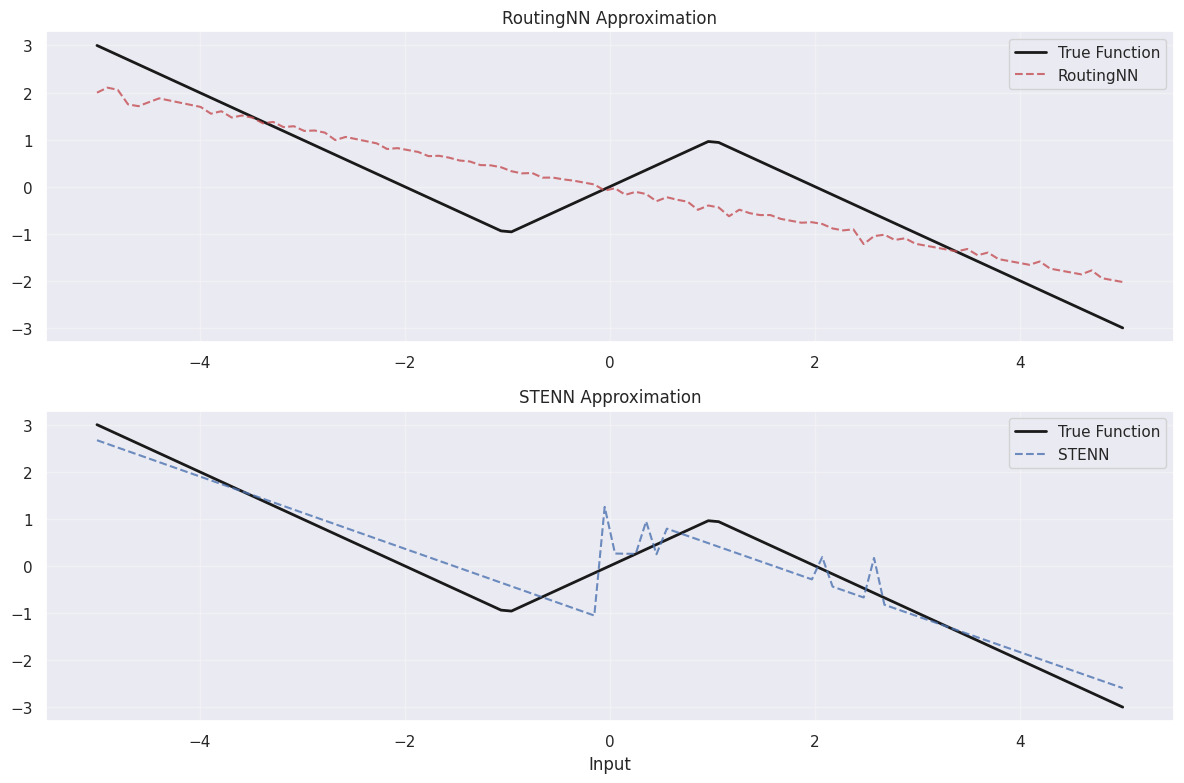
To test this out, I wrote a bunch of code that compares the routing layer above and the routing layer with the STE trick in learning this linear piecewise function: alt text

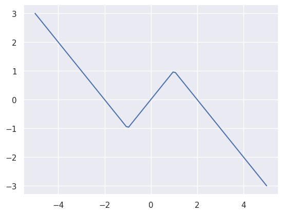
In this setup I have three experts, and each expert is a 1x1 linear projection. To learn this shape, the routing layer will need to route to the linear projection that corresponds to the right piece of the function.

Code

RoutingNN is unchanged from above. We add a new class, STERoutingLayer, which acts the same as above but uses the STE trick to update the routing weights.

import torch
from torch.nn import functional as F

class STERoutingLayer(torch.nn.Module):
    def __init__(self, model_dim, num_experts):
        super(STERoutingLayer, self).__init__()
        self.model_dim = model_dim
        self.num_experts = num_experts
        self.forward_proj = torch.nn.Linear(model_dim, num_experts)

    def forward(self, x):
        forward_proj = self.forward_proj(x)
        probs = F.softmax(forward_proj, dim=-1)
        chosen_expert = torch.multinomial(probs, 1)
        one_hot = F.one_hot(chosen_expert.squeeze(-1), num_classes=self.num_experts).float()
        ste_output = probs + (one_hot - probs).detach()
        return ste_output

class STEExpertLayer(torch.nn.Module):
    def __init__(self, model_dim, num_experts):
        super(STEExpertLayer, self).__init__()
        self.model_dim = model_dim
        self.num_experts = num_experts
        self.experts = torch.nn.ModuleList([torch.nn.Linear(model_dim, model_dim) for _ in range(num_experts)])

    def forward(self, x, chosen_expert_weights):
        expert_outputs = [expert(x) for expert in self.experts]
        return torch.sum(torch.stack(expert_outputs, dim = 1) * chosen_expert_weights.unsqueeze(-1), dim=1)
    
class STENN(torch.nn.Module):
    def __init__(self, model_dim, num_experts):
        super(STENN, self).__init__()
        self.routing_layer = STERoutingLayer(model_dim, num_experts)
        self.expert_layer = STEExpertLayer(model_dim, num_experts)

    def forward(self, x):
        chosen_expert = self.routing_layer(x)
        return self.expert_layer(x, chosen_expert)

Toy problem:

import matplotlib.pyplot as plt
import seaborn as sns
import numpy as np

def triangular_fn(x):
    if x < -1:
        return -x-2
    if x > 1:
        return 2-x
    return x

sns.set_theme()
plt.plot(np.linspace(-5, 5, 100), [triangular_fn(x) for x in np.linspace(-5, 5, 100)])
plt.show()

Training loop:

MODEL_DIM = 1
BATCH_SIZE = 32
NUM_EXPERTS = 3

# Training loop courtesy of Claude

# Check if CUDA is available and set device
device = torch.device('cuda' if torch.cuda.is_available() else 'cpu')
print(f"Using device: {device}")

# Generate training data for the triangular function
def generate_triangular_data(batch_size):
    x = torch.rand(batch_size, MODEL_DIM, device=device) * 10 - 5  # Sample uniformly from -5 to 5
    y = torch.tensor([triangular_fn(xi.item()) for xi in x.cpu()]).float().unsqueeze(-1).to(device)
    return x, y

# Training function
def train_model(model, num_steps=1000, lr=1e-2, plot_every=100):
    model = model.to(device)
    optimizer = torch.optim.Adam(model.parameters(), lr=lr)
    losses = []
    
    for step in range(num_steps):
        x, y = generate_triangular_data(BATCH_SIZE)
        
        optimizer.zero_grad()
        output = model(x)
        loss = torch.nn.functional.mse_loss(output, y)
        loss.backward()
        optimizer.step()
        
        losses.append(loss.item())
        
        if step % plot_every == 0:
            print(f"Step {step}, Loss: {loss.item():.4f}")
    
    return losses

# Train RoutingNN
print("Training RoutingNN...")
routing_model = RoutingNN(MODEL_DIM, NUM_EXPERTS)
routing_losses = train_model(routing_model, num_steps=2000)

# Train STENN
print("\nTraining STENN...")
ste_model = STENN(MODEL_DIM, NUM_EXPERTS)
ste_losses = train_model(ste_model, num_steps=2000)

# Plot training curves
plt.figure(figsize=(10, 6))
plt.plot(routing_losses, label='RoutingNN', alpha=0.7)
plt.plot(ste_losses, label='STENN', alpha=0.7)
plt.xlabel('Training Steps')
plt.ylabel('MSE Loss')
plt.title('Training Curves: RoutingNN vs STENN')
plt.legend()
plt.yscale('log')
plt.show()

# Test both models on a range of inputs
test_x = torch.linspace(-5, 5, 100, device=device).unsqueeze(-1)
true_y = torch.tensor([triangular_fn(x.item()) for x in test_x.cpu()])

with torch.no_grad():
    routing_pred = []
    ste_pred = []
    
    for x in test_x:
        routing_pred.append(routing_model(x.unsqueeze(0)).squeeze().cpu())
        ste_pred.append(ste_model(x.unsqueeze(0)).squeeze().cpu())
    
    routing_pred = torch.stack(routing_pred)
    ste_pred = torch.stack(ste_pred)

# Plot predictions
plt.figure(figsize=(12, 8))
plt.subplot(2, 1, 1)
plt.plot(test_x.cpu().squeeze(), true_y, 'k-', label='True Function', linewidth=2)
plt.plot(test_x.cpu().squeeze(), routing_pred, 'r--', label='RoutingNN', alpha=0.8)
plt.title('RoutingNN Approximation')
plt.legend()
plt.grid(True, alpha=0.3)

plt.subplot(2, 1, 2)
plt.plot(test_x.cpu().squeeze(), true_y, 'k-', label='True Function', linewidth=2)
plt.plot(test_x.cpu().squeeze(), ste_pred, 'b--', label='STENN', alpha=0.8)
plt.title('STENN Approximation')
plt.legend()
plt.grid(True, alpha=0.3)
plt.xlabel('Input')

plt.tight_layout()
plt.show()

The STE trick successfully guides the routing layer in modeling the triangular function:

alt text

At first glance, this appears strange. We apply a surrogate gradient to the backwards pass, causing the computed gradients to no longer be the true directions of steepest descent of the loss landscape. While the reason we must apply a surrogate gradient is because we have a nondifferentiable operation in our forwards pass (i.e it’s unsurprising that the gradient estimation approach outperforms an approach that leaves the non-differentiable layer unlearnable), the wide success of gradient estimation for SOTA models across domains is surprising.

Straight Through estimator is a magic door between cont/discrete. If people really cracked it at scale for 1.58 bits models, might be useful for all kinds of wild applications.
— Sasha Rush (@srush_nlp) April 1, 2024

Imagine we’re descending down a loss landscape. Instead of going in the direction that slopes steepest downhill, we check our GPS, which contains a totally different heightmap. Then we take a step in the downhill direction on the GPS map, which could mean in reality taking a step orthogonal to the slope or uphill.

The bias in the gradient estimator also affects all layers prior to the non-differentiable operation, as the surrogate gradient is part of their gradient flow as per the chain rule. This surrogate loss landscape must have some nice properties indeed such that the surrogate gradient direction matches the true one - if not in magnitude, then in direction.

What does the loss landscape look like?

The Loss Landscape

It’s difficult to compute the surrogate loss landscape, since we only interact with it via its gradient (and analytical integration methods terrify me). But we can still visualize the surrogate update steps we’d be taking at each point in the true loss landscape. Here, I’ve sampled a bunch of points on the loss landscape to form a surface and calculated the surrogate gradient (the little white cones).

While the surrogate gradient differs significantly from the true gradient, following the surrogate gradient (in this case) still yields convergence to the same minima.

This is a surprising empirical result and scales well, being used in modern VQ-VAEs and MoEs of billions of parameters. Theory has followed and yielded some justifications for STE’s efficacy.

Liu et al. 2023 prove that the STE, in expectation, is identical to the first-degree Taylor approximation of the true gradient:

\[E[\hat{\nabla}_{ST}] = \hat{\nabla}_{1st-order}\]

In our formulation, this would refer to:

\[E[\nabla_{i} L] = \nabla_p L_{1st-order}\]

or:

\[E\left[\frac{\partial L}{\partial p}\right] = \text{1st-order}\left(\frac{\partial L}{\partial y}\right)\]

Which implies that, in expectation, the gradients of the elements prior to the routing layer should at least have the same sign as the real gradient.

For their proof, see Appendix A of their paper.

Conclusion

The STE is a surprisingly robust approach for backpropagating through nondifferentiable functions. Have a stochastic variable in your neural network? No problem. In the backwards pass, pretend as if its gradient is the identity. Funnily enough, even Bengio called it a “heuristic method” when he reviewed it in 2013:

A fourth approach heuristically copies the gradient with respect to the stochastic output directly as an estimator of the gradient with respect to the sigmoid argument (we call this the straight-through estimator).

Modern works show that the STE is surprisingly robust, and works well when applied naively to a large variety of methods. While other gradient estimators expand upon STEs, they’re a simple and theory-backed baseline that we’ll build off (hopefully in similar posts in the future).

Note that the way I’ve formulated STEs allows it to be applied to random categorical variables. Using it for deterministic non-differentiable operations (e.g argmax) requires a bit more finesse, which I’ll discuss in the next post with Gumbel-Softmax.

alt text

yum.